Proceso de ortogonalización de Gram-Schmidt

De Wikipedia, la enciclopedia libre

En álgebra lineal, el proceso de ortogonalización de Gram–Schmidt es un algoritmo para construir, a partir de un conjunto de vectores de un espacio prehilbertiano (usualmente, el espacio euclídeo Rⁿ), otro conjunto ortonormal de vectores que genere el mismo subespacio vectorial.

Este algoritmo recibe su nombre de los matemáticos Jørgen Pedersen Gram y Erhard Schmidt.

Descripción del algoritmo de ortogonalización de Gram–Schmidt

Los dos primeros pasos del proceso de Gram–Schmidt

Se define, en primer lugar, el operador proyección mediante

$\mathrm{proj}_{\mathbf{u}}\,\mathbf{v} = {\langle \mathbf{v}, \mathbf{u}\rangle\over\langle \mathbf{u}, \mathbf{u}\rangle}\mathbf{u} = {||\mathbf{v}|| ||\mathbf{u}||\cos\alpha \over ||\mathbf{u}|| ||\mathbf{u}||1}\mathbf{u} = ||\mathbf{v}||\cos\alpha {\mathbf{u} \over ||\mathbf{u}||},$

donde los corchetes angulares representan el producto interior. Es evidente que

$\mathbf{v}-\mathrm{proj}_{\mathbf{u}}\,\mathbf{v}$

es un vector ortogonal a $\mathbf{u}$ . Entonces, dados los vectores $\mathbf{v}_1, \dots, \mathbf{v}_n$ , el algoritmo de Gram–Schmidt construye los vectores ortonormales $\mathbf{e}_1, \dots, \mathbf{e}_n$ de la manera siguiente:

	$\mathbf{u}_1 = \mathbf{v}_1,$		$\mathbf{e}_1 = {\mathbf{u}_1 \over \|\|\mathbf{u}_1\|\|}$
	$\mathbf{u}_2 = \mathbf{v}_2-\mathrm{proj}_{\mathbf{u}_1}\,\mathbf{v}_2,$		$\mathbf{e}_2 = {\mathbf{u}_2 \over \|\|\mathbf{u}_2\|\|}$
	$\mathbf{u}_3 = \mathbf{v}_3-\mathrm{proj}_{\mathbf{u}_1}\,\mathbf{v}_3-\mathrm{proj}_{\mathbf{u}_2}\,\mathbf{v}_3,$		$\mathbf{e}_3 = {\mathbf{u}_3 \over \|\|\mathbf{u}_3\|\|}$
	$\vdots$		$\vdots$
	$\mathbf{u}_k = \mathbf{v}_k-\sum_{j=1}^{k-1}\mathrm{proj}_{\mathbf{u}_j}\,\mathbf{v}_k,$		$\mathbf{e}_k = {\mathbf{u}_k\over\|\|\mathbf{u}_k\|\|}$

A partir de las propiedades de la proyección y del producto escalar, es sencillo probar que la sucesión de vectores $\mathbf{u}_1, \dots, \mathbf{u}_n$ es ortogonal.

Ejemplo

Considera el siguiente conjunto de vectores en R² (con el convencional producto interno)

$S = \left\lbrace\mathbf{v}_1=\begin{pmatrix} 3 \\ 1\end{pmatrix}, \mathbf{v}_2=\begin{pmatrix}2 \\2\end{pmatrix}\right\rbrace.$

Ahora, aplicamos Gram–Schmidt, para obtener un conjunto de vectores ortogonales:

$\mathbf{u}_1=\mathbf{v}_1=\begin{pmatrix}3\\1\end{pmatrix}$

$\mathbf{u}_2 = \mathbf{v}_2 - \mathrm{proj}_{\mathbf{u}_1} \, \mathbf{v}_2 = \begin{pmatrix}2\\2\end{pmatrix} - \mathrm{proj}_{({3 \atop 1})} \, {\begin{pmatrix}2\\2\end{pmatrix}} = \begin{pmatrix} -2/5 \\6/5 \end{pmatrix}.$

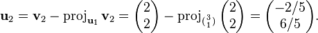
Verificamos que los vectores u₁ y u₂ son de hecho ortogonales:

$\langle\mathbf{u}_1,\mathbf{u}_2\rangle = \left\langle \begin{pmatrix}3\\1\end{pmatrix}, \begin{pmatrix}-2/5\\6/5\end{pmatrix} \right\rangle = -\frac65 + \frac65 = 0.$